Adventures of a self-learning data scientist - My first pull request: imfr

I changed code to work under imfr Version 2.

My first pull request

Package ‘imfr’ is the first package which merged my very small pull request. Thank you, creator Christopher Gandrud. I would like to show a usage example below.

Code

library(tidyverse)
library(imfr)

theme_set(theme_light())

Look for database ID

Package ‘imfr’ provides some functions to help us explore IMF database. First, I use ‘imf_databases’ function to get database IDs.

Code

imf_app_name("mitsuoxv")

databases <- imf_databases()

There are 323 databases. I get a dataframe with 2 columns, ‘database_id’ and ‘description’.

Code

head(databases)

  database_id
1 BOP_2017M06
2  BOP_2020M3
3 BOP_2017M11
4  DOT_2020Q1
5  GFSMAB2016
6 BOP_2019M12
                                                                       description
1                                              Balance of Payments (BOP), 2017 M06
2                                              Balance of Payments (BOP), 2020 M03
3                                              Balance of Payments (BOP), 2017 M11
4                                    Direction of Trade Statistics (DOTS), 2020 Q1
5 Government Finance Statistics Yearbook (GFSY 2016), Main Aggregates and Balances
6                                              Balance of Payments (BOP), 2019 M12

I transform ‘description’ into all lower characters, in order to make search easier.

Code

databases <- databases |> 
  mutate(description = str_to_lower(description))

As I am interested in debt issues, I search ‘debt’ in ‘description’. I get ‘database_id’ HPDD, of which ‘description’ is historical public debt.

Code

databases |> 
  filter(str_detect(description, "debt"))

  database_id                   description
1        HPDD historical public debt (hpdd)

Retrieve parameters of a database

I use ‘imf_parameters’ function to retrieve the parameters of the database whose id is HPDD.

Code

params <- imf_parameters("HPDD")

str(params)

List of 3
 $ freq     :'data.frame':  3 obs. of  2 variables:
  ..$ input_code : chr [1:3] "A" "M" "Q"
  ..$ description: chr [1:3] "Annual" "Monthly" "Quarterly"
 $ ref_area :'data.frame':  199 obs. of  2 variables:
  ..$ input_code : chr [1:199] "AF" "AL" "DZ" "AO" ...
  ..$ description: chr [1:199] "Afghanistan" "Albania" "Algeria" "Angola" ...
 $ indicator:'data.frame':  1 obs. of  2 variables:
  ..$ input_code : chr "GGXWDG_GDP"
  ..$ description: chr "Debt to GDP Ratio"

There are 3 lists of code and description:

frequency,
geographical areas (code: two-letter country codes defined in ISO 3166-1), and
indicator. Here, I get only one indicator GGXWDG_GDP, which describes Debt to GDP Ratio.

Download data

Now I am ready to download data. I use ‘imf_dataset’ function. I specify HPDD as ‘database_id’, select ‘freq’, ‘ref_area’ and ‘indicator’ from the parameters, and set ‘start_year’ and ‘end_year’.

Code

debt_gdp_ratio <- imf_dataset(
  database_id = "HPDD",
  freq = "A",
  ref_area = params$ref_area$input_code,
  indicator = "GGXWDG_GDP",
  start_year = 1700, end_year = 2020
)

I change ‘year’ from character to integer, and add ‘country’ by utilizing the 2nd list.

Code

debt_gdp_ratio <- debt_gdp_ratio |> 
  as_tibble() |> 
  mutate(across(date:value, as.numeric)) |> 
  select(date:ref_area) |> 
  left_join(params$ref_area, by = c("ref_area"="input_code")) |> 
  rename(country = description)

head(debt_gdp_ratio)

# A tibble: 6 × 5
   date value freq  ref_area country
  <dbl> <dbl> <chr> <chr>    <chr>  
1  1994  85.2 A     AL       Albania
2  1995  75.0 A     AL       Albania
3  1996  76.7 A     AL       Albania
4  1997  81.9 A     AL       Albania
5  1998  71.9 A     AL       Albania
6  1999  63.9 A     AL       Albania

Some countries have data as old as 1800. They are U.K., U.S. and Sweden. Most recent year is 2015.

Code

range(debt_gdp_ratio$date)

[1] 1800 2015

Code

debt_gdp_ratio |>  
  filter(date == 1800)

# A tibble: 3 × 5
   date value freq  ref_area country       
  <dbl> <dbl> <chr> <chr>    <chr>         
1  1800  34.3 A     SE       Sweden        
2  1800 177.  A     GB       United Kingdom
3  1800  18.1 A     US       United States

191 countries have some data.

A chart and some thoughts

I use countrycode.org to get two-letter code of the select countries, and draw a chart.

Debt to GDP ratio rises in the war, and, if you win, it decreases thanks to growth and inflation. If you lose, it decreases thanks to some defaults and very high inflation. Some people in the losing side lose their financial wealth, but most misery does not come from debt, but from physical devastation.

Recently it rises due to secular stagnation, in which monetary policy is constrained by zero lower bound of nominal interest rates, and full employment can be achieved only by bubble or expansionary fiscal policy.

Code

debt_gdp_ratio %>% 
  filter(ref_area %in% c("US", "GB", "JP", "ZW")) %>% 
  ggplot(aes(date, value, color = fct_reorder2(country, date, value))) +
  geom_line(linewidth = 1) +
  labs(x = NULL, y = "Debt to GDP Ratio",
       color = "counry")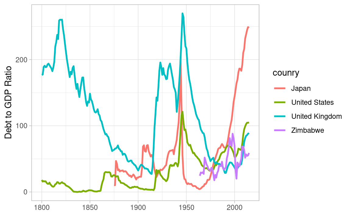

Figure 1: Debt to GDP Ratio in Japan, the US, the UK and Zimbabwe

Debt to GDP ratio reflects the government capacity to borrow, the household and the enterprise capacity to save, and the financial sector capacity to mediate. It melts, if nominal GDP growth rates are higher than nominal interest rates.

If Japan falls into deflation, nominal GDP growth rates are negative, and nominal interest rates are zero due to lower bound. This leads to ballooning debt to GDP ratios. Austerity is not the solution, as it leads to deeper deflation and under-employment. Coordinating and rebalancing the monetary and fiscal policies is the solution, which can make inflation expectation positive and well anchored.