Code
library(tidyverse)
library(OECD)
library(janitor)
library(countrycode)
library(ggrepel)

theme_set(theme_light())library(tidyverse)
library(OECD)
library(janitor)
library(countrycode)
library(ggrepel)
theme_set(theme_light())Prof Masayuki Morikawa at Hitotsubashi University published an article titled “We should emphasize soft infrastructure in government expenditures to enhance productivity” (Japanese) in “Lecture on Economics” in Nikkei news paper on February 10, 2022. In his article he shows the chart which I will soon replicate, and suggests that higher debt may reduce economic growth rates.
I follow “Alternative data-acquisition strategy” in https://github.com/expersso/OECD.
# GDP per hour worked, constant prices
productivity <- get_dataset("PDB_GR",
                    filter = "AUS+AUT+BEL+CAN+CHL+COL+CZE+DNK+EST+FIN+FRA+DEU+GRC+HUN+ISL+IRL+ISR+ITA+JPN+KOR+LVA+LTU+LUX+MEX+NLD+NZL+NOR+POL+PRT+SVK+SVN+ESP+SWE+CHE+TUR+GBR+USA.T_GDPHRS_V.2015Y",
                    start_time = 2008,
                    end_time = 2019,
                    pre_formatted = TRUE) %>%
  clean_names()

prod_growth <- productivity %>%
  mutate(obs_value = as.numeric(obs_value)) %>%
  filter(time %in% c("2008", "2019")) %>%
  select(location, time, obs_value) %>%
  pivot_wider(names_from = time, values_from = obs_value) %>%
mutate(prod_growth = (`2019` / `2008`)^(1/11) * 100 - 100)gdp <- get_dataset("SNA_TABLE1",
filter = "AUS+AUT+BEL+CAN+CHL+COL+CRI+CZE+DNK+EST+FIN+FRA+DEU+GRC+HUN+ISL+IRL+ISR+ITA+JPN+KOR+LVA+LTU+LUX+MEX+NLD+NZL+NOR+POL+PRT+SVK+SVN+ESP+SWE+CHE+TUR+GBR+USA.GDP+B1GVO_Q+B1GVR_U+P119+D21_D31+D21S1+D31S1+DB1_GA+B1_GE+P3_P5+P3+P31S14_S15+P31S14+P31S15+P3S13+P31S13+P32S13+P41+P5+P51+P51N1111+P51N1112+P51N1113+P51N11131+P51N11132+P51N1113I+P51N1113O+P51N1114+P51N112+P52_P53+P52+P53+B11+P6+P61+P62+P7+P71+P72+DB1_GE+B1_GI+D1+D1A_B+D1C_E+D1D+D1F+D1G_I+D1J_K+D1L_P+D1VA+D1VB_E+D1VC+D1VF+D1VG_I+D1VJ+D1VK+D1VL+D1VM_N+D1VO_Q+D1VR_U+D11+D11A_B+D11C_E+D11D+D11F+D11G_I+D11J_K+D11L_P+D11VA+D11VB_E+D11VC+D11VF+D11VG_I+D11VJ+D11VK+D11VL+D11VM_N+D11VO_Q+D11VR_U+D12+D12VA+D12VB_E+D12VC+D12VF+D12VG_I+D12VJ+D12VK+D12VL+D12VM_N+D12VO_Q+D12VR_U+B2G_B3G+D2_D3+D2S1+D3S1+DB1_GI.V+VIXOB+DOB+G",
start_time = 2008,
end_time = 2019,
pre_formatted = TRUE) %>%
clean_names()
gdp_growth <- gdp %>%
mutate(obs_value = as.numeric(obs_value)) %>%
filter(transact == "B1_GE", measure == "V",
time %in% c("2008", "2019")) %>%
select(location, time, obs_value) %>%
pivot_wider(names_from = time, values_from = obs_value) %>%
mutate(gdp_growth = (`2019` / `2008`)^(1/11) * 100 - 100) %>%
select(location, gdp_growth)As Columbia and Turkey don’t have complete 12 data from 2008 to 2019 in general government debts per GDP, I drop them.
gov <- get_dataset("GOV",
                    filter = "AUS+AUT+BEL+CAN+CHL+COL+CRI+CZE+DNK+EST+FIN+FRA+DEU+GRC+HUN+ISL+IRL+ISR+ITA+JPN+KOR+LVA+LTU+LUX+MEX+NLD+NZL+NOR+POL+PRT+SVK+SVN+ESP+SWE+CHE+TUR+GBR+USA.GGD_GDP+GTR_GDP+GTE_GDP+GINV_GDP",
                    start_time = 2008,
                    end_time = 2019,
                    pre_formatted = TRUE) %>%
  clean_names()

gov %>%
  filter(ind == "GGD_GDP") %>%
  group_by(cou) %>%
  summarize(n = n()) %>%
  filter(n != 12) # drop "COL", "TUR"
# A tibble: 2 × 2
cou n
<chr> <int>
1 COL 5
2 TUR 10ggd_gdp <- gov %>%
mutate(obs_value = as.numeric(obs_value)) %>%
filter(ind == "GGD_GDP", !cou %in% c("COL", "TUR")) %>%
group_by(cou) %>%
summarize(ggd_gdp = mean(obs_value), .groups = "drop_last") %>%
rename(location = cou)He draws a scatter plot of government debts per GDP and economic growth rates from 2008 to 2019 (probably selected as the year of full employment) in OECD members.
Although he cautions that the relationship is correlation, not causation, he says that high government debts may reduce economic growth.
Although he labels only Japan, Greece, Italy, France, Germany, United Kingdom and United States in the chart in his article, I label all countries here.
gdp_growth %>%
  left_join(ggd_gdp, by = "location") %>%
  mutate(
    country = countrycode(location, origin = "iso3c", destination = "country.name")) %>%
  ggplot(aes(ggd_gdp, gdp_growth)) +
  geom_hline(yintercept = 0, color = "white", size = 1.5) +
  geom_point() +
  geom_smooth(method = "lm", se = FALSE) +
  geom_text_repel(aes(label = country)) +
  scale_y_continuous(breaks = -3:5) +
  labs(x = "Average gross government debt per GDP (percent)",
       y = "Average real GDP growth rates (percent)",
       title = "Replication of the chart in the article",
       subtitle = "from 2008 to 2019",
       caption = "Source: OECD")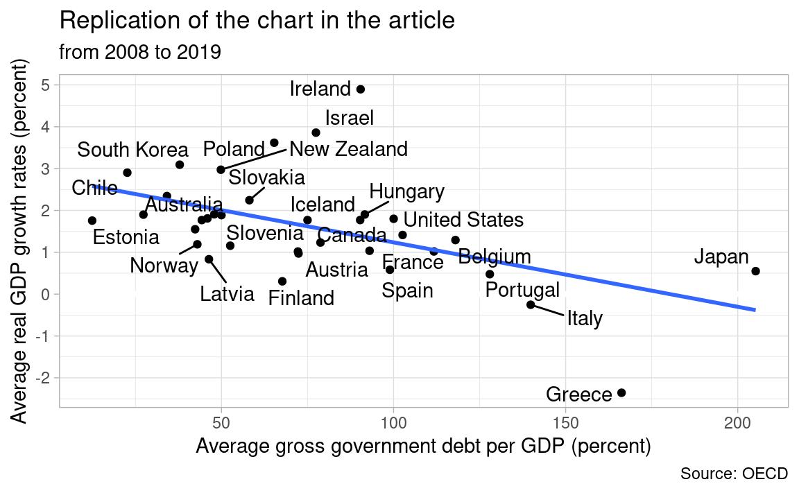
As this article is about how to enhance productivity by fiscal expentitures, and Japan economic growth is suffering from decreasing population and labor force, I replace economic growth rates with productivity (GDP per hours worked) growth rates. The slope of the linear regression line is now flatter.
prod_growth %>%
  left_join(ggd_gdp, by = "location") %>%
  mutate(
    country = countrycode(location, origin = "iso3c", destination = "country.name")) %>%
  ggplot(aes(ggd_gdp, prod_growth)) +
  geom_hline(yintercept = 0, color = "white", size = 1.5) +
  geom_point() +
  geom_smooth(method = "lm", se = FALSE) +
  geom_text_repel(aes(label = country)) +
  scale_y_continuous(breaks = -3:5) +
  labs(x = "Average gross government debt per GDP (percent)",
       y = "Average productivity growth rates (percent)",
       title = "Differences narrow based on productivity growth rates",
       subtitle = "from 2008 to 2019",
       caption = "Source: OECD")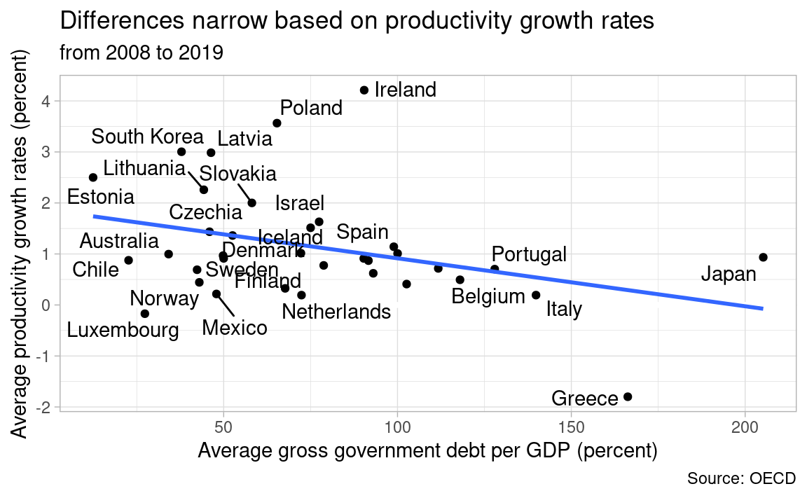
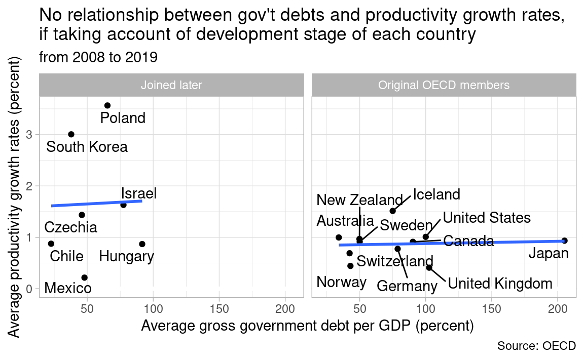
As Euro countries, like Greece and Italy, don’t borrow in its own currency but in the euro, and were forced into austerity by Germany from 2008 to 2019, I exclude Euro countries except Germany. I also exclude Denmark as its currency is pegged to the euro. As a result, I just consider the relationship between gov’t debts in its own currency and productivity growth.
I also separate the OECD countries by whether they are the original members or not, to take account of the development stages by each country.
Now there is no relationship between gov’t debts and productivity growth. Am I cherry picking the data? I believe not.
euro_cou <- c("AUT", "BEL", "NLD", "FIN", "FRA", "IRL", "ITA", "LUX",
                     "PRT", "ESP", "GRC", "SVN", "CYP", "MLT", "SVK", "EST",
                     "LVA", "LTU", "DNK")

prod_growth %>%
  filter(!location %in% euro_cou) %>%
  mutate(original_member = if_else(
    location %in% c("MEX", "CZE", "HUN", "POL", "KOR", "CHL",
                    "ISR"), "Joined later", "Original OECD members"
  )) %>%
  left_join(ggd_gdp, by = "location") %>%
  mutate(
    country = countrycode(location, origin = "iso3c", destination = "country.name")) %>%
  ggplot(aes(ggd_gdp, prod_growth)) +
  geom_hline(yintercept = 0, color = "white", size = 1.5) +
  geom_point() +
  geom_smooth(method = "lm", se = FALSE) +
  geom_text_repel(aes(label = country)) +
  scale_y_continuous(breaks = -3:5) +
  facet_wrap(vars(original_member)) +
  labs(x = "Average gross government debt per GDP (percent)",
       y = "Average productivity growth rates (percent)",
       title = "No relationship between gov't debts and productivity growth rates,\nif taking account of development stage of each country",
       subtitle = "from 2008 to 2019",
       caption = "Source: OECD")