Code
library(tidyverse)
library(lubridate)
library(patchwork)

library(scales)
theme_set(theme_light())

library(OECD)
library(gghighlight)library(tidyverse)
library(lubridate)
library(patchwork)
library(scales)
theme_set(theme_light())
library(OECD)
library(gghighlight)Prof Tetsuji Okazaki of the University of Tokyo shows Japan lags the US in labor productivity level, and the gap is widening, in his “Lecture on Economics” in Nikkei news paper on February 17, 2023 (Japanese).
countries <- c("USA", "JPN", "GBR", "DEU", "FRA", "ITA", "CAN")

exchange_rate <- get_dataset(
  "SNA_TABLE4",
  filter = list(countries, c("PPPGDP")),
  start_time = 2005, end_time = 2021
) |>
  mutate(across(c(ObsValue, Time), as.numeric))

gdp <- get_dataset(
  "SNA_TABLE1",
  filter = list(countries, "B1_GE", c("DOB", "C", "V")),
  start_time = 2005, end_time = 2021
) |>
  mutate(across(c(ObsValue, Time), as.numeric))

labor <- get_dataset(
  "ALFS_SUMTAB",
  filter = list(countries, "YGTT08L1_ST"),
  start_time = 2005, end_time = 2021
) |>
  mutate(across(c(ObsValue, Time), as.numeric))

hours_worked <- get_dataset(
  "ANHRS",
  filter = list(countries, "TE"),
  start_time = 2005, end_time = 2021
) |>
mutate(across(c(ObsValue, Time), as.numeric))us_deflator <- gdp |>
filter(LOCATION == "USA", MEASURE == "DOB") |>
mutate(deflator = ObsValue / 100) |>
select(Time, deflator)
employment <- labor |>
select(LOCATION, Time, employment = ObsValue)
ppp <- exchange_rate |>
select(LOCATION, Time, ppp = ObsValue)ppp_method <- gdp |>
filter(MEASURE == "C") |>
left_join(employment, by = c("LOCATION", "Time")) |>
left_join(ppp, by = c("LOCATION", "Time")) |>
left_join(us_deflator, by = "Time") |>
mutate(
nominal_prod_loc = ObsValue / employment,
nominal_prod_usd = nominal_prod_loc / ppp,
real_prod_usd = nominal_prod_usd / deflator
) |>
group_by(LOCATION) |>
mutate(index = real_prod_usd / real_prod_usd[1] * 100) |>
ungroup()
p1 <- ppp_method |>
filter(LOCATION %in% c("USA", "JPN")) |>
mutate(LOCATION = factor(LOCATION, levels = c("USA", "JPN"))) |>
ggplot(aes(Time, real_prod_usd)) +
geom_line(aes(color = LOCATION)) +
labs(x = NULL, y = "Real productivity per person\n(thousand dollars, PPP, 2015 price)",
color = "Country")
p2 <- ppp_method |>
filter(LOCATION %in% c("USA", "JPN")) |>
mutate(LOCATION = factor(LOCATION, levels = c("USA", "JPN"))) |>
ggplot(aes(Time, index)) +
geom_line(aes(color = LOCATION)) +
scale_y_continuous(limits = c(85, 125)) +
labs(x = NULL, y = "Real productivity per person\n(2005 = 100)",
color = "Country")hours_worked_te <- hours_worked |>
select(COUNTRY, Time, hours_worked = ObsValue)
non_ppp_method <- gdp |>
filter(MEASURE == "V") |>
left_join(employment, by = c("LOCATION", "Time")) |>
left_join(hours_worked_te, by = c("LOCATION" = "COUNTRY", "Time")) |>
mutate(
real_prod_loc = ObsValue / employment,
real_prod_loc_hr = real_prod_loc / hours_worked
) |>
group_by(LOCATION) |>
mutate(
prod_per_person = real_prod_loc / real_prod_loc[1] * 100,
prod_per_hour = real_prod_loc_hr / real_prod_loc_hr[1] * 100
) |>
ungroup()
p3 <- non_ppp_method |>
filter(LOCATION %in% c("USA", "JPN")) |>
mutate(LOCATION = factor(LOCATION, levels = c("USA", "JPN"))) |>
ggplot(aes(Time, prod_per_person)) +
geom_line(aes(color = LOCATION)) +
geom_line(aes(y = index), color = "gray80",
data = ppp_method |> filter(LOCATION == "JPN")) +
scale_y_continuous(limits = c(85, 125)) +
labs(x = NULL, y = "Real productivity per person\n(2005 = 100)",
color = "Country")
p4 <- non_ppp_method |>
filter(LOCATION %in% c("USA", "JPN")) |>
mutate(LOCATION = factor(LOCATION, levels = c("USA", "JPN"))) |>
ggplot(aes(Time, prod_per_hour)) +
geom_line(aes(color = LOCATION)) +
scale_y_continuous(limits = c(85, 125)) +
labs(x = NULL, y = "Real productivity per hour\n(2005 = 100)",
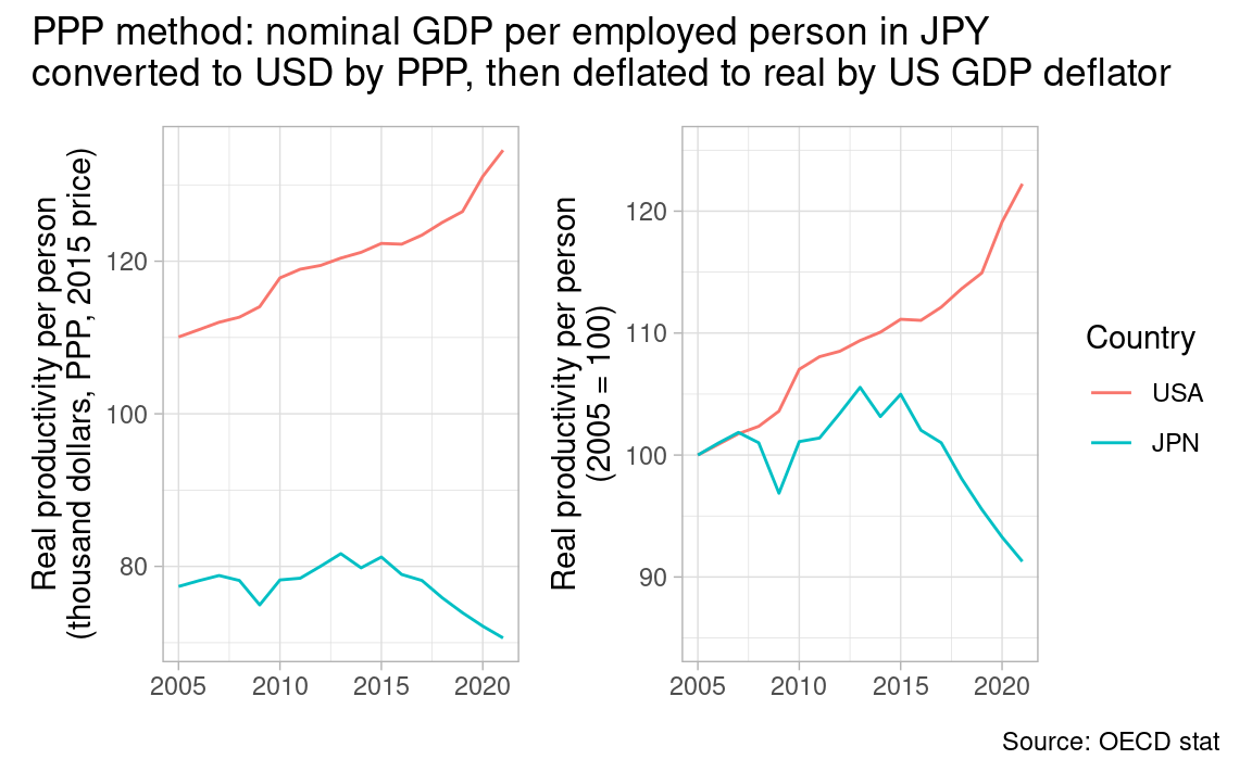
color = "Country")He shows the chart which is not exactly same, but similar to the left chart below, and says the gap in labor productivity level between the US and Japan is widening. I have modified it to make the right chart so that 2005 = 100. He uses PPP method. I think it is very difficult or impossible to compare the productivity level, as Japan and the US produce very different products and services. It is only possible to compare productivity growth, then using PPP is unnecessary and inappropriate.
p1 + p2 + plot_layout(ncol = 2, guides = "collect") + plot_annotation(
  title = "PPP method: nominal GDP per employed person in JPY\nconverted to USD by PPP, then deflated to real by US GDP deflator",
  caption = "Source: OECD stat"
)
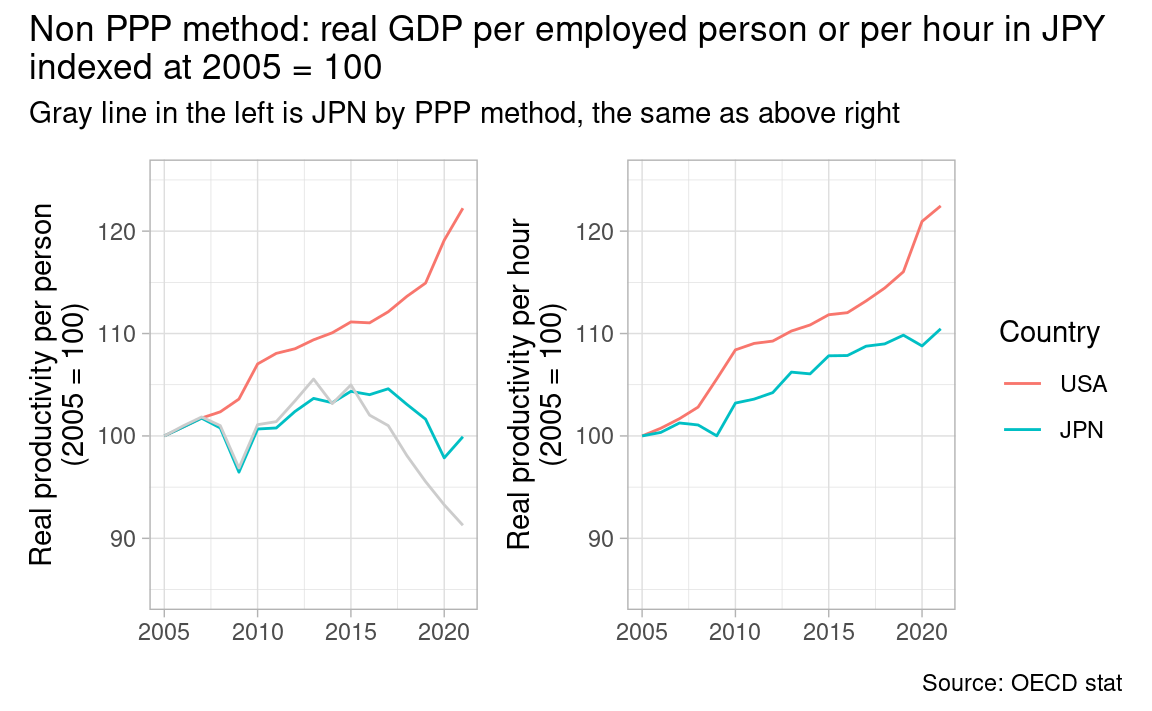
Below is the estimates of labor productivity growth without using PPP. Growth gap narrows in the left below. If we look at productivity per hour instead of per person in the right below, the gap narrows even further.
p3 + p4 + plot_layout(ncol = 2, guides = "collect") + plot_annotation(
  title = "Non PPP method: real GDP per employed person or per hour in JPY \nindexed at 2005 = 100",
  subtitle = "Gray line in the left is JPN by PPP method, the same as above right",
  caption = "Source: OECD stat"
)
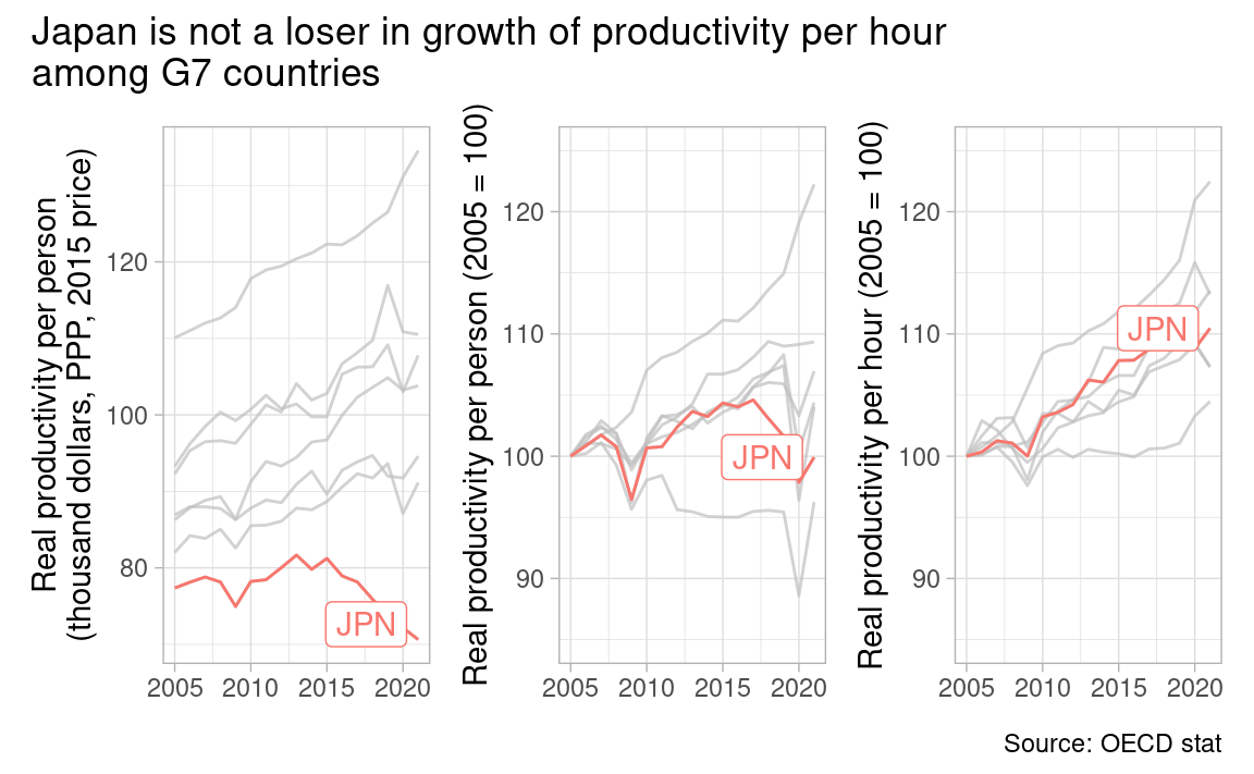
Although Japan looks like a loser in productivity per person in PPP dollars, it is not a loser in growth of productivity per hour.
p5 <- ppp_method |>
  ggplot(aes(Time, real_prod_usd)) +
  geom_line(aes(color = LOCATION)) +
  gghighlight(LOCATION == "JPN", use_group_by = FALSE) +
  labs(x = NULL, y = "Real productivity per person\n(thousand dollars, PPP, 2015 price)",
       color = "Country")

p6 <- non_ppp_method |>
  ggplot(aes(Time, prod_per_person)) +
  geom_line(aes(color = LOCATION)) +
  gghighlight(LOCATION == "JPN", use_group_by = FALSE) +
  scale_y_continuous(limits = c(85, 125)) +
  labs(x = NULL, y = "Real productivity per person (2005 = 100)",
       color = "Country")

p7 <- non_ppp_method |>
  ggplot(aes(Time, prod_per_hour)) +
  geom_line(aes(color = LOCATION)) +
  gghighlight(LOCATION == "JPN", use_group_by = FALSE) +
  scale_y_continuous(limits = c(85, 125)) +
  labs(x = NULL, y = "Real productivity per hour (2005 = 100)",
       color = "Country")

p5 + p6 + p7 + plot_layout(ncol = 3, guides = "collect") + plot_annotation(
  title = "Japan is not a loser in growth of productivity per hour\namong G7 countries",
  caption = "Source: OECD stat"
)