Code
library(tidyverse)
library(readxl)
library(tsibble)
library(lubridate)
library(patchwork)
library(tidyquant)

theme_set(theme_light())library(tidyverse)
library(readxl)
library(tsibble)
library(lubridate)
library(patchwork)
library(tidyquant)
theme_set(theme_light())fred_data <- tq_get(c("GASREGW", "WCOILWTICO", "WCOILBRENTEU"),
get = "economic.data", from = "2003-01-01") %>%
mutate(week = yearweek(date)) %>%
select(-date) # USD per gallon
us_data <- fred_data %>%
filter(symbol == "GASREGW") %>%
select(week, price_incl_tax = price) %>%
mutate(price = price_incl_tax - 0.184 - 0.50)
uk_data <- read_csv("data/CSV_040422.csv",
skip = 2) %>%
select(1, 2, 4, 6) %>%
setNames(c("week", "price_incl_tax", "duty", "vat_rate")) %>%
mutate(
week = dmy(week),
week = yearweek(week),
price = price_incl_tax / (1 + vat_rate / 100) - duty
) %>%
select(week, price_incl_tax, price) # pence per litre
retail <- read_excel("data/220406s5.xls",
sheet = "レギュラー",
col_types = c("text", "date", rep("text", 59)))
jp_data <- retail %>%
slice_head(n = nrow(retail) - 1) %>%
select(date = "調査日", price_incl_tax = "全 国") %>%
mutate(
date = as.Date(date),
price_incl_tax = as.numeric(price_incl_tax)
) %>%
filter(date >= "2003-01-01") %>%
mutate(
vat_rate = case_when(
date < "2004-04-01" ~ 0,
date < "2014-04-01" ~ .05,
date < "2019-10-01" ~ .08,
TRUE ~ .1
),
price = price_incl_tax / (1 + vat_rate) - 53.8,
week = yearweek(date)
) %>%
select(week, price_incl_tax, price) # yen per litre
brent <- fred_data %>%
filter(symbol == "WCOILBRENTEU") %>%
mutate(
country = "Brent",
price_incl_tax = price
) %>%
select(-symbol)
combo <- bind_rows(us_data %>% mutate(country = "United States"),
uk_data %>% mutate(country = "United Kingdom"),
jp_data %>% mutate(country = "Japan"),
brent) %>%
mutate(date = as.Date(week))Nikkei reported on April 7, 2022 that the subsidy to wholesalers, which began in late January, led to less rapid rise of gasoline prices in Japan than the US, the UK, Germany and France, and that this price-control policy may distort the economy.
Although I agree to the opposition to price-control, I think this Nikkei article has two problems.
Below left, I replicate the chart in the Nikkei article, though I add Brent crude oil prices, and omit Germany and France, as I can’t get those data.
The problem of this chart is that prices include taxes. In the most recent week, taxes occupy 19 percent in the US, 49 percent in the UK, and 40 percent in Japan. The more shares taxes occupy, the less prices can change.
Below right, I remove taxes. The US approaces to Brent, and the UK approaches to US. However, Japan still lags behind. Is this thanks to METI’s subsidy? No, I would like to claim Japan usually lags behind.
p1 <- combo %>%
filter(date >= as.Date("2022-01-01"), date < as.Date("2022-04-07")) %>%
  group_by(country) %>%
  mutate(index = price_incl_tax / first(price_incl_tax) * 100) %>%
  ungroup() %>%
  ggplot(aes(week, index, color = country)) +
  geom_line(size = 1) +
  scale_x_yearweek(date_label = "%m/\n%d", date_break = "1 month") +
  ylim(90, 160) +
  theme(panel.grid.minor.x = element_blank()) +
  labs(x = NULL, y = "Index (Jan 3, 2022 = 100)",
       color = NULL,
       title = "Gasoline prices\nincluding taxes")
Warning: Using `size` aesthetic for lines was deprecated in ggplot2 3.4.0.
ℹ Please use `linewidth` instead.p2 <- combo %>%
filter(date >= as.Date("2022-01-01"), date < as.Date("2022-04-07")) %>%
group_by(country) %>%
mutate(index = price / first(price) * 100) %>%
ungroup() %>%
ggplot(aes(week, index, color = country)) +
geom_line(size = 1) +
scale_x_yearweek(date_label = "%m/\n%d", date_break = "1 month") +
ylim(90, 160) +
theme(panel.grid.minor.x = element_blank()) +
labs(x = NULL, y = NULL,
color = NULL,
title = "Gasoline prices\nexcluding taxes")
p1 + p2 + plot_layout(guides = "collect")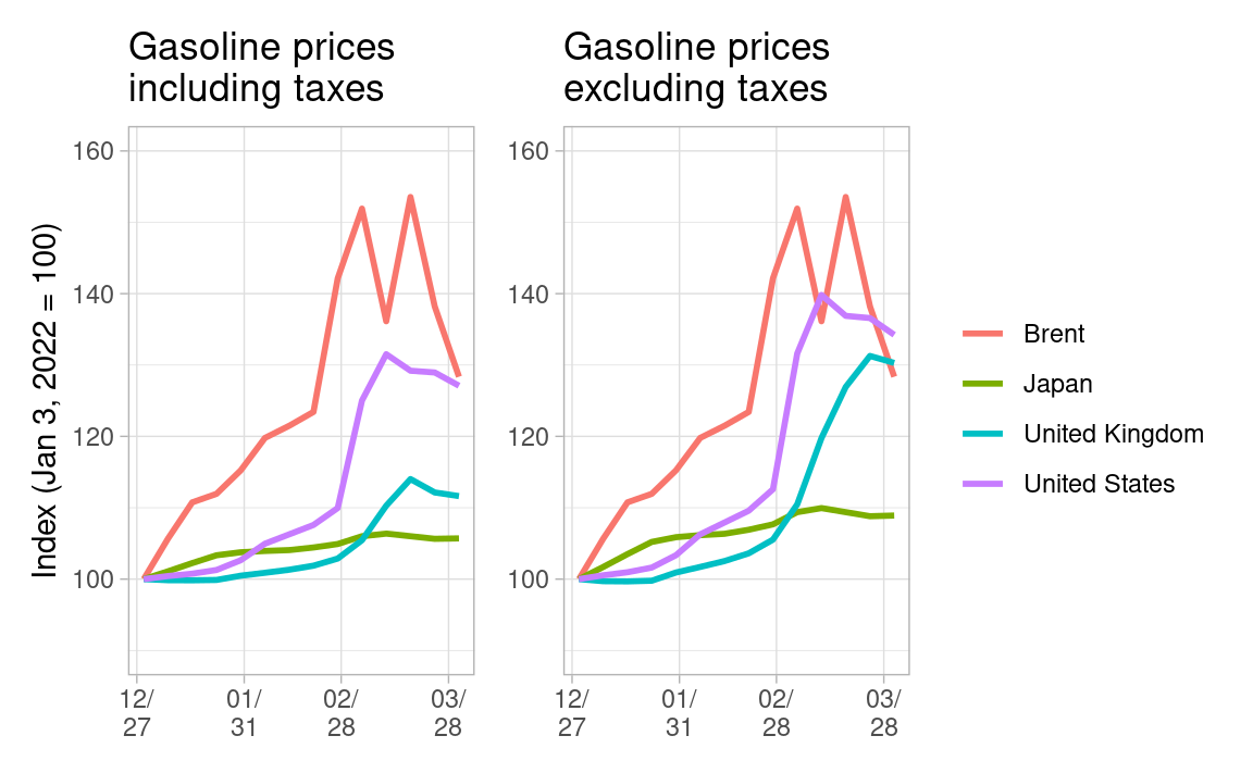
To support my claim, I must use weekly data of crude oil prices. As I can’t get Dubai prices, I use Brent prices. Basically crude oil prices are global, so it should not be a problem when I use Brent instead of Dubai.
fred_data %>%
  filter(symbol %in% c("WCOILWTICO", "WCOILBRENTEU")) %>%
  mutate(symbol = recode(symbol,
                         "WCOILWTICO" = "WTI",
                         "WCOILBRENTEU" = "Brent")) %>%
  ggplot(aes(week, price, color = symbol)) +
  geom_line(size = 1) +
  scale_x_yearweek(date_label = "%Y") +
  labs(x = NULL, y = "USD per barrel", color = NULL,
       title = "Crude oil prices (weekly)")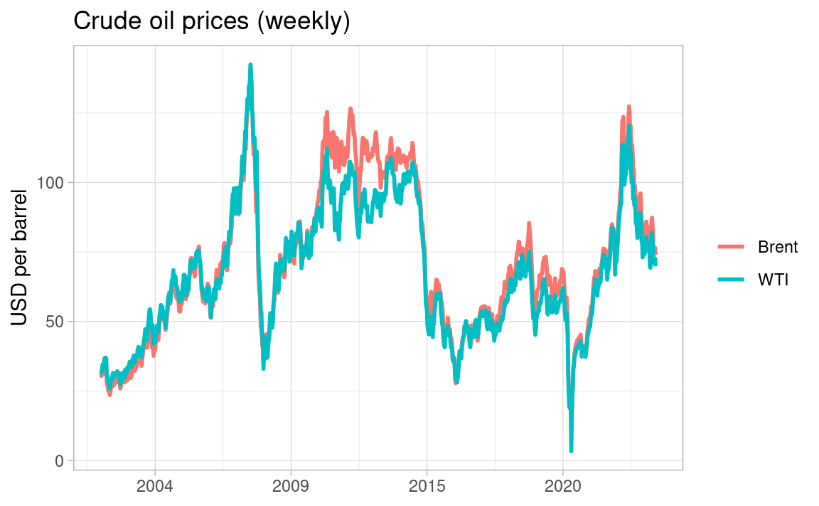
Nikkei states that price rise in Japan is suppressed, thanks to subsidies by METI. Really? I doubt it.
When I compared wholesale gasoline prices with imported crude oil prices in February 2022, I could not find the evidence that the subsidy lowered wholesale prices. Refer to my GitHub page.
I even suspect the subsidy raised prices, as METI shows suggested retail prices, which is responsive to Dubai prices and incorporate historically high margin between Dubai prices and retail prices, every week. As METI’s counterfactual retail prices without sibsidy reflect Dubai prices of 2 weeks ago, they are as volatile as Dubai prices.
As you see below, retail prices in Japan were less responsive to changes of crude oil prices than the US and the UK. Look at rise, fall and rise again from 2007 to 2009, you see Japan lags Brent both in rise and fall. You can see the same pattern in 2020. In rise of 2021, Japan still lags, though it catches up to Brent in the end.
I can say wholesalers in Japan were slow to raise, and slow to cut prices in the past. I guess it’s because Japan imports crude oil mainly from Middle East, one month carrying distance away, while the US and the UK produce crude oil domestically. However, wholesalers are now quick to raise, thanks to METI’s subsidy, but slow to cut prices as usual, unless monitored by METI.
draw_by_year <- function(year) {
  df <- combo %>%
    filter(date >= as.Date(paste0(year, "-01-01")),
           date <= as.Date(paste0(year + 1, "-01-01")))

  first_date = df %>%
    head(1) %>%
    pull(date)

  df %>%
    group_by(country) %>%
    mutate(index = price / first(price) * 100) %>%
    ungroup() %>%
    ggplot(aes(week, index, color = country)) +
    geom_line(size = 1) +
    scale_x_yearweek(date_label = "%b") +
    theme(panel.grid.minor.x = element_blank()) +
    labs(x = NULL, y = paste0(first_date, " = 100"),
         color = NULL,
         title = as.character(year))
}

charts <- vector("list", length(2004:2021))
charts <- map(2004:2021, draw_by_year)

p_charts <- charts[[1]] + charts[[2]] + charts[[3]] +
  charts[[4]] + charts[[5]] + charts[[6]] +
  charts[[7]] + charts[[8]] + charts[[9]] +
  charts[[10]] + charts[[11]] + charts[[12]] +
  charts[[13]] + charts[[14]] + charts[[15]] +
  charts[[16]] + charts[[17]] + charts[[18]]

p_charts + plot_layout(ncol = 3, guides = "collect")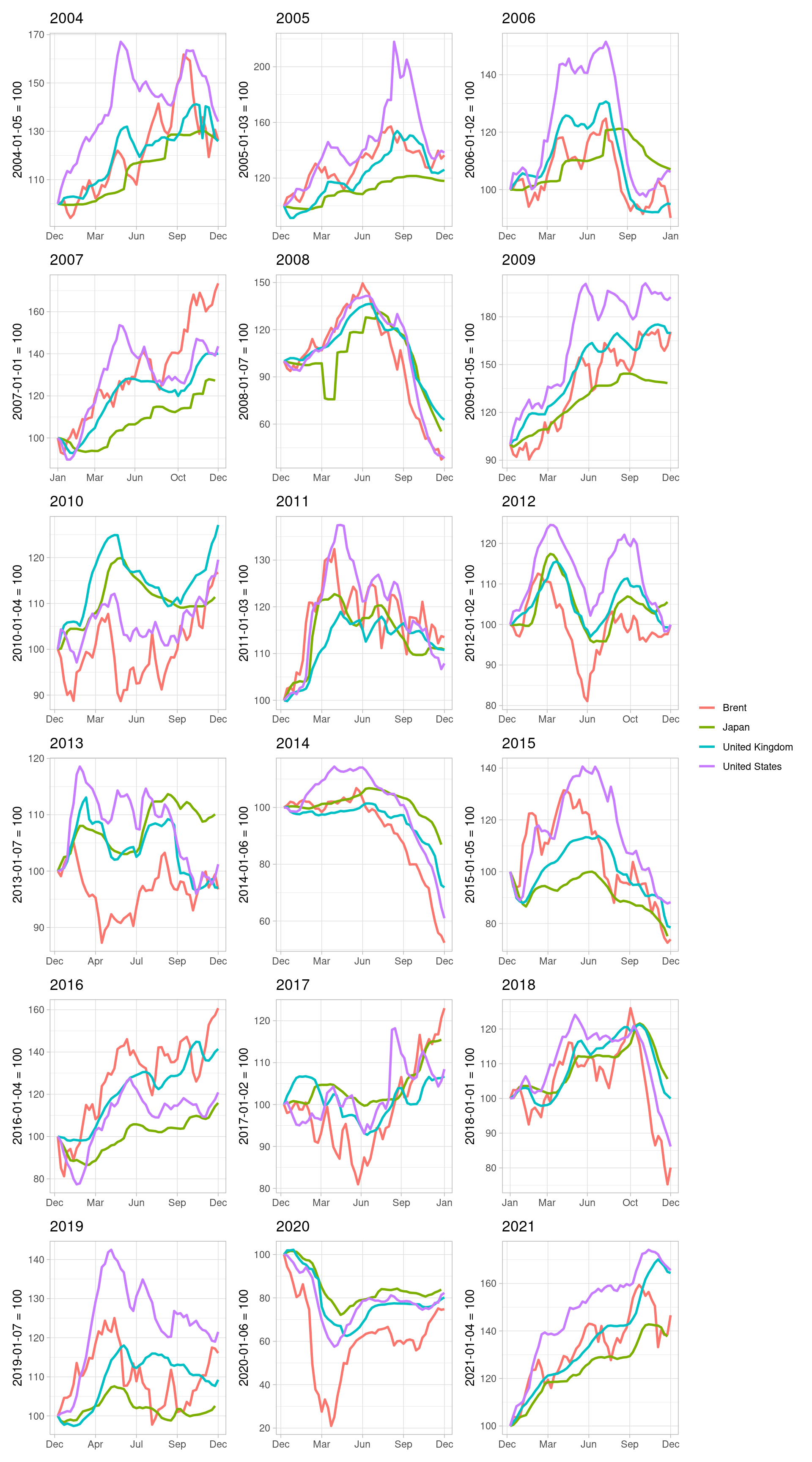
P.S.
I learned the title of this post, “quick to raise, but slow to cut gas prices”, is called “rockets and feathers” in the US from Paul Krugman’s blog post.