Code
library(tidyverse)
library(readxl)

theme_set(theme_light())library(tidyverse)
library(readxl)
theme_set(theme_light())read_dat1 <- function(url, sheet, year) {
# download
tf <- tempfile(fileext = ".xls")
httr::GET(url, httr::write_disk(tf))
# read
dat <- read_excel(tf, sheet = sheet)
ratios <- dat[5, 9] %>%
as.numeric()
names(ratios) <- year
# return
ratios
}
read_dat2 <- function(url, sheet1, sheet2, year) {
# download
tf <- tempfile(fileext = ".xls")
httr::GET(url, httr::write_disk(tf))
# read
dat1 <- read_excel(tf, sheet = sheet1)
sales <- as.numeric(dat1[4, 12]) * 100
dat2 <- read_excel(tf, sheet = sheet2)
costs <- as.numeric(dat2[6, 6])
ratios <- costs / sales * 100
names(ratios) <- year
# return
ratios
}
read_dat3 <- function(url, sheet1, r1, c1, sheet2, r2, c2, year) {
# download
tf <- tempfile(fileext = ".xls")
httr::GET(url, httr::write_disk(tf))
# read
dat1 <- read_excel(tf, sheet = sheet1)
sales <- as.numeric(dat1[r1, c1])
dat2 <- read_excel(tf, sheet = sheet2)
costs <- parse_number(as.character(dat2[r2, c2]))
ratios <- costs / sales * 100
names(ratios) <- year
# return
ratios
}
read_dat4 <- function(url, sheet1, r1, c1, sheet2, r2, c2, year) {
# download
tf <- tempfile(fileext = ".xlsx")
httr::GET(url, httr::write_disk(tf))
# read
dat1 <- read_excel(tf, sheet = sheet1)
sales <- as.numeric(dat1[r1, c1])
dat2 <- read_excel(tf, sheet = sheet2)
costs <- parse_number(as.character(dat2[r2, c2]))
ratios <- costs / sales * 100
names(ratios) <- year
# return
ratios
}dat <- rep(NA_real_, 27)
dat[1] <- read_dat1("https://www.e-stat.go.jp/stat-search/file-download?statInfId=000031365960&fileKind=0", 8, 1994)
dat[2] <- read_dat1("https://www.e-stat.go.jp/stat-search/file-download?statInfId=000031365902&fileKind=0", 10, 1995)
dat[3] <- read_dat2("https://www.e-stat.go.jp/stat-search/file-download?statInfId=000031365900&fileKind=0", 2, 11, 1996)
dat[4] <- read_dat3("https://www.e-stat.go.jp/stat-search/file-download?statInfId=000031365898&fileKind=0", 8, 4, 3, 11, 5, 6, 1997)
dat[5] <- read_dat3("https://www.e-stat.go.jp/stat-search/file-download?statInfId=000002335269&fileKind=0", 16, 4, 3, 19, 6, 6, 1998)
dat[6] <- read_dat3("https://www.e-stat.go.jp/stat-search/file-download?statInfId=000002335267&fileKind=0", 15, 4, 3, 18, 6, 6, 1999)
dat[7] <- read_dat3("https://www.e-stat.go.jp/stat-search/file-download?statInfId=000002335264&fileKind=0", 16, 4, 3, 19, 6, 6, 2000)
dat[8] <- read_dat3("https://www.e-stat.go.jp/stat-search/file-download?statInfId=000002335251&fileKind=0", 16, 4, 3, 19, 6, 6, 2001)
dat[9] <- read_dat3("https://www.e-stat.go.jp/stat-search/file-download?statInfId=000002335238&fileKind=0", 6, 4, 3, 9, 6, 6, 2002)
dat[10] <- read_dat3("https://www.e-stat.go.jp/stat-search/file-download?statInfId=000002335227&fileKind=0", 5, 4, 3, 8, 6, 6, 2003)
dat[11] <- read_dat3("https://www.e-stat.go.jp/stat-search/file-download?statInfId=000002335186&fileKind=0", 6, 5, 6, 9, 6, 6, 2004)
dat[12] <- read_dat3("https://www.e-stat.go.jp/stat-search/file-download?statInfId=000002335198&fileKind=0", 5, 5, 3, 8, 6, 6, 2005)
dat[13] <- read_dat3("https://www.e-stat.go.jp/stat-search/file-download?statInfId=000002332496&fileKind=0", 5, 4, 3, 8, 6, 6, 2006)
dat[14] <- read_dat3("https://www.e-stat.go.jp/stat-search/file-download?statInfId=000008797328&fileKind=0", 5, 5, 3, 8, 6, 6, 2007)
dat[15] <- read_dat3("https://www.e-stat.go.jp/stat-search/file-download?statInfId=000008862770&fileKind=0", 5, 4, 3, 8, 6, 6, 2008)
dat[16] <- read_dat3("https://www.e-stat.go.jp/stat-search/file-download?statInfId=000012448588&fileKind=0", 5, 4, 3, 8, 6, 6, 2009)
dat[17] <- read_dat3("https://www.e-stat.go.jp/stat-search/file-download?statInfId=000031364720&fileKind=0", 5, 4, 3, 8, 6, 6, 2010)
dat[18] <- read_dat3("https://www.e-stat.go.jp/stat-search/file-download?statInfId=000031364766&fileKind=0", 5, 4, 3, 8, 6, 6, 2011)
dat[19] <- read_dat3("https://www.e-stat.go.jp/stat-search/file-download?statInfId=000031364844&fileKind=0", 5, 4, 3, 8, 6, 6, 2012)
dat[20] <- read_dat3("https://www.e-stat.go.jp/stat-search/file-download?statInfId=000031364750&fileKind=0", 5, 4, 3, 8, 6, 6, 2013)
dat[21] <- read_dat3("https://www.e-stat.go.jp/stat-search/file-download?statInfId=000031435520&fileKind=0", 5, 4, 3, 8, 6, 6, 2014)
dat[22] <- read_dat3("https://www.e-stat.go.jp/stat-search/file-download?statInfId=000031626692&fileKind=0", 5, 4, 3, 8, 6, 6, 2015)
dat[23] <- read_dat3("https://www.e-stat.go.jp/stat-search/file-download?statInfId=000031735887&fileKind=0", 5, 4, 3, 8, 6, 6, 2016)
dat[24] <- read_dat3("https://www.e-stat.go.jp/stat-search/file-download?statInfId=000031841099&fileKind=0", 5, 4, 3, 8, 6, 6, 2017)
dat[25] <- read_dat3("https://www.e-stat.go.jp/stat-search/file-download?statInfId=000031974813&fileKind=0", 5, 4, 3, 8, 6, 6, 2018)
dat[26] <- read_dat4("https://www.e-stat.go.jp/stat-search/file-download?statInfId=000032116539&fileKind=0", 5, 6, 4, 8, 7, 7, 2019)
dat[27] <- read_dat3("https://www.e-stat.go.jp/stat-search/file-download?statInfId=000032210740&fileKind=0", 5, 6, 4, 8, 7, 7, 2020)Mr. Shunsuke Kobayashi, Chief Economist of Mizuho Securities, said that high cost of goods sold per sales ratio, 80 percent according to METI business activity survey, is the evidence that businesses could not transfer an increase in commodity and materials costs to sales price, in the evening NHK program “Close-up Gendai” on October 3.
I was surprised that he says 80% is high. So I get METI business activity survey data from e-stat, and plot from fiscal year 1994 to 2020 as below. FY 2020 is the most recent one. As there is no upward trend, 80% in FY 2020 is not high compared to the past.
tibble(
  year = 1994:2020,
  sales_cost_ratio = dat
) %>%
  ggplot(aes(year, sales_cost_ratio)) +
  geom_line() +
  scale_y_continuous(limits = c(0, 100), breaks = seq(0, 100 , 20),
                     expand = c(0, 0)) +
  labs(x = NULL, y = "Cost of goods sold to sales ratios (%)",
       title = "No upward trend in COGS to sales ratios up to FY 2020",
       caption = "Source: METI business activity survey")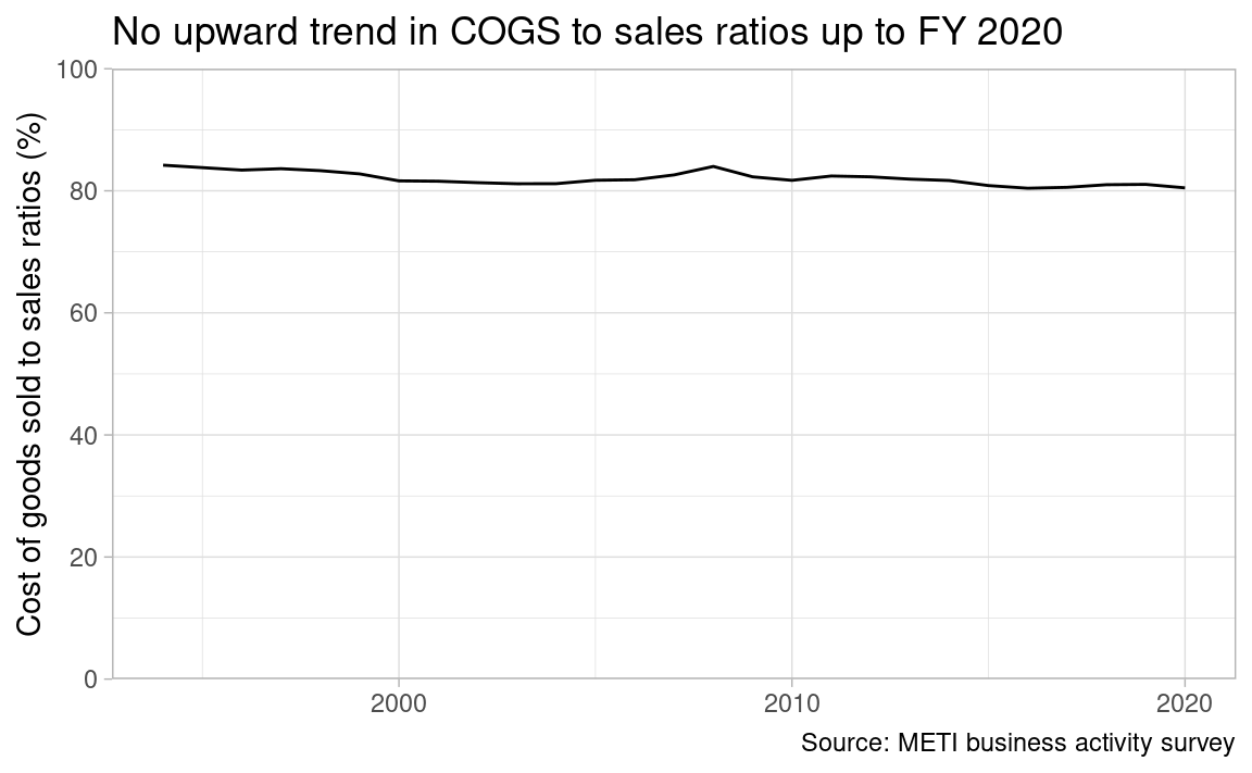
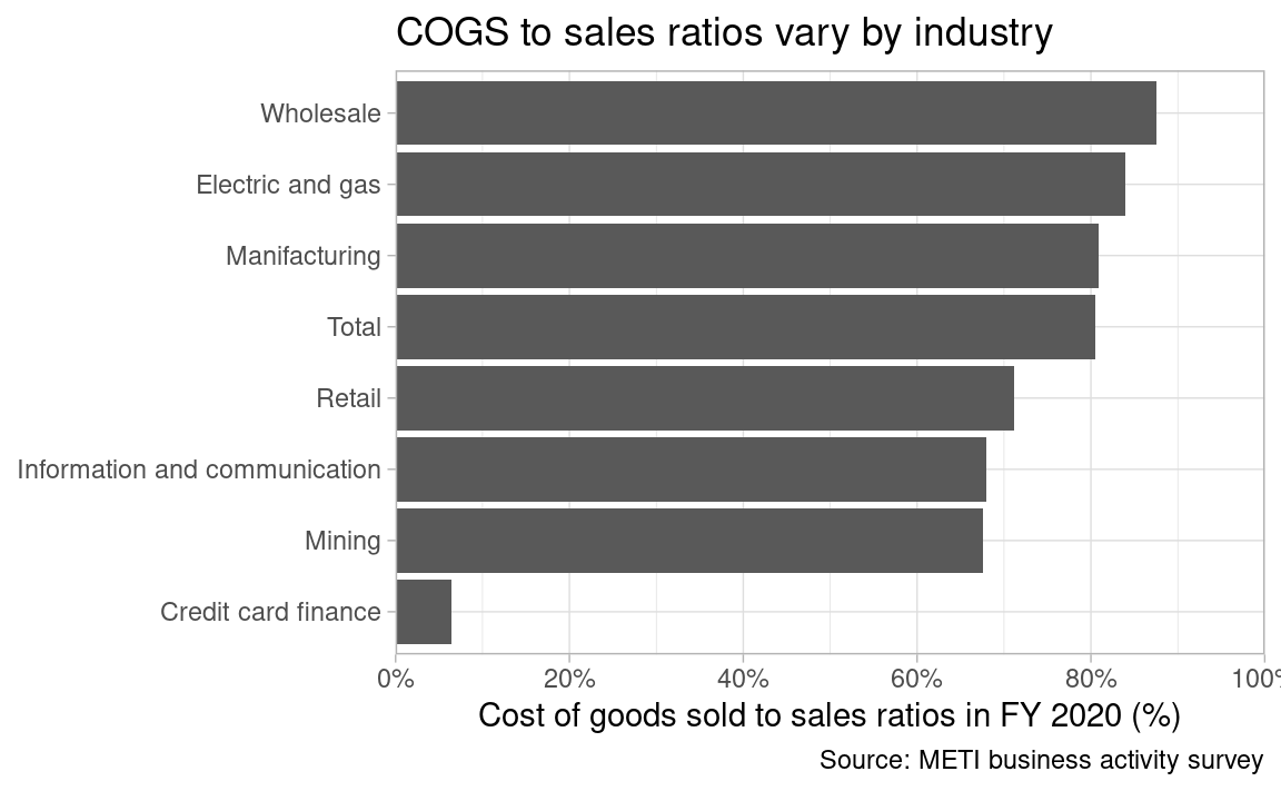
He may have considered 80% is high, when compared to some foreign countries. But this number, COGS to sales ratio in total, is not appropriate for cross-country comparison, because industrial structure, corporate structure and counting method matter. In a country where just one company produces and sells goods in a country, COGS to sales ratio in total will be very low. In another country where many divided companies transact each other, it will be higher. In addition, as COGS to sales ratios vary by industry as below, composition of industries effects total ratio.
url <- "https://www.e-stat.go.jp/stat-search/file-download?statInfId=000032210740&fileKind=0"

# download
tf <- tempfile(fileext = ".xls")

httr::GET(url, httr::write_disk(tf))# read
dat1 <- read_excel(tf, sheet = 5, skip = 5)
dat2 <- read_excel(tf, sheet = 8, skip = 6)
dat_2020 <- bind_cols(dat1[, c(1:2, 4)], dat2[, 7])
names(dat_2020) <- c("code", "industry_j", "sales", "cogs")dat_2020 %>%
mutate(ratio = cogs / sales) %>%
filter(code %in% c("000", "C", "E", "F", "G", "I1", "I2", "J1")) %>%
mutate(
industry_e = c("Total", "Mining", "Manifacturing", "Electric and gas", "Information and communication", "Wholesale", "Retail", "Credit card finance"),
industry_e = fct_reorder(industry_e, ratio)
) %>%
ggplot(aes(ratio, industry_e)) +
geom_col() +
scale_x_continuous(labels = scales::percent,
limits = c(0, 1),
breaks = seq(0, 1, 0.2),
expand = c(0, 0)) +
labs(y = NULL, x = "Cost of goods sold to sales ratios in FY 2020 (%)",
title = "COGS to sales ratios vary by industry",
caption = "Source: METI business activity survey")